From 0 to Bi(ge)nius: "Basic maths"

Thanks a lot to Oba, Nuliel, Hyunmin, Ali, Nico and Jim for the review ❤️
Feel free to DM me on Twitter: @0xteddav if you find mistakes in this article or if you have any question.

Binius is a new way to build SNARKs by Benjamin Diamond and Jim Posen (from Irreducible). It uses “towers of binary fields” (yes, it sounds complicated but it should become obvious by the end of this article) and a variation of the Hyperplonk IOP over binary fields, combined with the Brakedown polynomial commitment scheme for better prover efficiency.
Here’s the paper: Succinct Arguments over Towers of Binary Fields.
If you didn’t understand anything of what I just said, don’t worry. I will explain it all in simple terms so that the proof system is -hopefully- clear by the end of the series 🙏
This first part will start with the basics. We’re going to look at what “small fields” are, then we’ll get to field extensions and finally reach the “towers”.

Small fields: Goldilocks, Mersenne

Big fields (think $>2^{256}$) are used in elliptic-curve-based SNARKs in order to ensure high levels of bit security.
On the other hand, hash-based STARKs can afford to use smaller fields (think $2^{64}$ or even $2^{32}$), leading to significant gains in prover efficiency.
But the crucial part in verification is sampling a random number r from the field and checking “some” equality at r. If the field is too small, the prover could trick the verifier. That’s where extension fields come in: most of the operations will be done in the small fields while some operations are moved to the larger extension field. We will get into the details later in the article.
I’m going to assume that you know what a prime field is. If you don’t, stop here and Google it 🔍
What we call “small field” is basically just taking a smaller prime (yes, $2^{64}$ is “small”) and reducing every number modulo that prime.
For example, the “Goldilocks field” (I don’t know why it’s named this way) uses $p=2^{64}-2^{32}+1$ while “Mersenne31” uses $p=2^{31}-1$.
When doing modular math using these fields, any number will be less than 64 and 31 bits for Goldilocks and Mersenne31, respectively.

Why small fields?

The idea is simple: make things faster!
Generating a ZK proof takes a lot of computational power: due to the modular math operations, to interpolate, and evaluate polynomials. Researchers have been trying to improve that.
Small fields speed things up by:

• taking better advantage of our processors, which are 64 bits, so they are way more optimized for numbers smaller than 64 bits.
• optimizing the memory used. That’s what you’ll find as “embedding overhead”: the bigger the field, the more memory is used to store that number

When working in fields, everything has to be reduced “modulo p”. The naive way to do modulo would be something like:

result = a - (a // b) * b

Which requires a division… then a multiplication… and a subtraction 😱 that’s a lot! Of course we can optimize things with Montgomery or Barrett reduction for example.
Performing these operations with small numbers is fast (because of lower memory usage, and better hardware optimization), but it becomes a burden when working with big numbers. The computational cost is roughly proportional to the number of bits of the modulo.
Working with small numbers makes it possible to use lookup tables and avoid mathematical operations altogether. For an intuition on why, imagine each table row as the concatenation of a||b||result the formula above. If the field is small enough, we could commit to all possible values of the table and then simply prove a certain row is in the table -which achieves the same goal as evaluating the above formula.
According to Polygon’s blog post on plonky2: “simply using Goldilocks’s 64-bit field instead of a 256-bit field improved proving speed by 40x”.
If we reduce our field to the binary field $\mathbb{F}_2$, which is what Binius is doing, there is no modular reduction needed at all! We’ll come back to it later, but the main idea is:

• addition is an XOR:
  • 0 + 0 = 0
  • 1 + 0 = 1
  • 1 + 1 = 0
• multiplication is an AND:
  • 0 * 0 = 0
  • 1 * 0 = 0
  • 1 * 1 = 1

How practical are binary fields?

Ok great, but we might still need to use bigger values. We don’t want to lose precision. Let’s say we are working with a modulo p = 101 but we want to express a list of salaries, so we need our values to go up to $10000, it would be a shame to reduce everything mod 101.
So what is usually done is to use “limbs”, which means we divide our “big” number into an array of smaller numbers. An example?
We want to express 5863: [5, 58]
Each limb is mod p and we just have to multiply each limb by $p^i$ (where i is the index).
So $5863 = 5*p^0+58*p^1$
With python we can easily find these numbers:

a = 5863 % 101
b = 5863 // 101

Working with numbers smaller than p? No problem.
Big numbers? split them up into small limbs.
It might sound a bit crude, but in practice most numbers are really small (ex: lots 0/1 booleans), so the gains are huge.

Extension fields

As I told you before, we need to “extend” our field…
At first I couldn’t understand any of it 🤯 but if I wanted to write about Binius, unfortunately, I couldn’t avoid it…
My goal, dear reader, is to save you as much time by explaining what I learned in simple terms 😘
The best explanation for me was Ben Edgington’s “BLS12-381 For The Rest Of Us” article. You should definitely read it!
In this section we’ll be using a finite prime field $\mathbb{F}_p$ (our “base field”) where p = 7.
Why? No reason… Most tutorials use 3 and 5 so I wanted a different example 😄 In the next section we’ll finally get to our beloved “binary field”.

Definition

In $\mathbb{F}_7$ there are only 7 numbers (0 to 6) to play with, but we want to extend our field so that we can have more fun.
That’s where it becomes a bit confusing. In “field extensions”, we don’t use integers, we represent our values with polynomials. The base field stays the same (7), which means that every coefficient of our polynomial will be reduced modulo 7.
Yes, that’s confusing…
If we take a degree 3 extension, this is what values look like now: $ax^2+bx+c$ , where a, b and c are modulo 7. Our field is now $\mathbb{F}_{7^3}$.
The idea is that every number (the coefficients) stays in the base field, so optimizations that I talked about previously still work. And multiplying polynomials is very efficient (using the Karatsuba algorithm or the Fast Fourier Transform for example).
Just to warn you: I’m going to use u instead of x in when representing polynomials. It doesn’t change anything, but it will make things more clear for when we introduce new variables later in the article (yes, it’s going to get more complicated…). So instead of writing $ax^2+bx+c$ , I will write $au^2+bu+c$ . Basically I want to use $u, v , w$ for variables instead of $x, y, z$.
Let’s see a real example to see how that works.

Our first extension: quadratic $^2$

We are going to create a quadratic (degree 2) extension. Our extended field is now $\mathbb{F}_{7^2}$ and you guessed it, you can now fit 49 values in there 🤩
If m is the degree of our extension, then the maximum degree of each polynomial is m - 1.
So here, each polynomial will have the form: $a_1*u+a_0$ where $a_1$ and $a_0$ are in our field $\mathbb{F}_7$ (so modulo 7).
Just to make sure it’s clear, here’s the list of all the possibilities we now have (I used chatgpt to write the polynomials to save time 😊):
Prompt: can you write for me all the linear polynomials where coefficients are between 0 and 6 (included)
Certainly! Linear polynomials are of the form: f(x)=ax+b where a and b are coefficients. Given that the coefficients a and b can take any integer value from 0 to 6, we can list all possible combinations of a and b.
There are 7 possible values for each coefficient, so we have 7×7=49 possible polynomials. Here they are: 0x+0,0x+1,0x+2,0x+3,0x+4,0x+5,0x+6,1x+0,1x+1,1x+2,1x+3,1x+4,1x+5,1x+6,2x+0,2x+1,2x+2,2x+3,2x+4,2x+5,2x+6,3x+0,3x+1,3x+2,3x+3,3x+4,3x+5,3x+6,4x+0,4x+1,4x+2,4x+3,4x+4,4x+5,4x+6,5x+0,5x+1,5x+2,5x+3,5x+4,5x+5,5x+6,6x+0,6x+1,6x+2,6x+3,6x+4,6x+5,6x+6

Irreducible polynomial

We’re just missing one thing: an irreducible polynomial.
Irreducible means that it has no root in $\mathbb{F}_7$, and also that it cannot be factored into the product of two polynomials of lower degree.
If we multiply 2 values, we could end up with a degree 2 polynomial, so we need a way to “stay in our field”. That means reducing values modulo the “irreducible polynomial”.

Polynomial modulo polynomial

How do we find that irreducible polynomial? And what does it mean to “reduce a polynomial modulo another polynomial”.
For the first question, we’ll just use Sage to make it easy to find an irreducible polynomial in our field

p = 7

F7 = GF(p)
R.<u> = F7[]

for f in R.polynomials(of_degree=2):
    if f.is_irreducible():
        print(f)

It found 126 possibilities 😨 here are the first ones:

u^2 + 1
u^2 + 2
u^2 + 4
u^2 + u + 3
u^2 + u + 4
u^2 + u + 6
u^2 + 2*u + 2
...

We’re going to use $u^2+1$ for our first example.
Let’s pick a crazy random polynomial: $30 u^3 + 126 u^2 + 144 u + 24$
First remember that our coefficients are modulo 7, so we reduce that. We end up with:
$2u^3 + 0u^2 + 4u + 3 = 2u^3 + 4u + 3$

The generic algorithm for a modulo is the same I gave you before: result = a - (a // b) * b.
We have $A(u)=2u^3+4u+3$ and $B(u)=u^2+1$ and we want to compute A(u) % B(u).
The steps would be:

1. Divide the leading term of A(u) by the leading term of B(u)
2. Multiply the result by B(u)
3. Subtract this product from A(u)
4. Repeat until the degree of the remainder is less than the degree of B(u)

But I’m going to give you a simple technique to do that manually: we can replace B(u) in A(u).
So just replace $u^2$ by $-1$ in $A(u)$. And since we are modulo 7, that means “replace $u^2$ by 6”:
$A(u) \mod B(u) = 2(u^2*u)+4u+3=2*(6*u)+4u+3=12u+4u+3=16u+3=2u+3$

p = 7

F7 = GF(p)
R.<u> = F7[]

A = R(30*u^3 + 126*u^2 + 144*u + 24)
B = R(u^2 + 1)

print(A)
print(A % B)

# 2*u^3 + 4*u + 3
# 2*u + 3

That was easy, right?

Switch base group

I’m going to try something: let’s just use the same polynomial but change our base field and try again.
This is just for fun, and (most importantly) to make sure everything that everything we learned up until now is clear in our heads.
Instead of working in $\mathbb{F}_7$ we’ll switch to $\mathbb{F}_{11}$. So now coefficients are mod 11.
Our polynomial $A(u)=30 u^3 + 126 u^2 + 144 u + 24$ becomes $A(u)= 8u^3 + 5u^2 + u + 2$
Using Sage we can find many irreducible polynomials, I decided to use: $B(u) = 4u^2 + 10u + 3$, why not?
And our result is finally: $A(u) \mod B(u) = 5u+5$
How?

• First we isolate $u^2$ in B(u): $4u^2=-10u-3=u+8$ (remember, we’re modulo 11)
  $u^2=\frac{u+8}{4}$
  So we need the inverse of 4 in $\mathbb{F}_{11}$. We can use python, which gives us 3 (pow(4,-1,11))
  So $u^2=3u+24=3u+2$

• Then we can replace in A(u):
  $A(u)\mod B(u) = 8u*u^2 + 5u^2 + u + 2=8u(3u+2)+5(3u+2)+u+2$
  $A(u)\mod B(u) = 24u^2+16u+15u+10+u+2=2u^2+10u+1$
  $A(u)\mod B(u) = 2(3u+2)+10u+1=6u+4+10u+1=5u+5$

Now you’re a pro 🥳🥳🥳 We can continue!

Back to our extension

Let’s get back to our initial settings now and play in $\mathbb{F}_{7^2}$.
Previously we used the irreducible polynomial $u^2+1$, but from now on, let’s use $u^2+u+3$. I want to make things more spicy… 😈
Let’s say we multiply 2 values:
$a=3u+2$
$b=4u+5$
→ $a*b=12u^2+23u+10$

First we reduce our coefficients modulo 7 → $5u^2+2u+3$
That’s where we use our irreducible polynomial! We can now reduce and make it “fit” in our field:
$5u^2+2u+3 \mod (u^2+u+3) = 4u+2$
And that’s it! In our extension field $\mathbb{F}_{7^2}$ : $(3u+2)(4u+5)=4u+2$
Like we did before, we could do that manually by replacing $u^2$ with $-u-3=6u+4$
→ $5*(6u+4)+2u+3=30u+20+2u+3=32u+23=4u+2$

Mental representation

At first I tried to represent values in extension fields as integers because I was getting confused by the polynomials. But it’s a bad idea.
If you tried to do that here, you would have:

• a = 23 (3*7+2)
• b = 33 (4*7+5)
• the result is 30 (4*7+2)

Which doesn’t make too much sense… because the result actually depends on the irreducible polynomial we chose.
So if you really wanted to use integers, you could say that: in $\mathbb{F}_{7^2}[u]/u^2+u+3$ , we have: 23*33=30
But just stop thinking about it, and embrace the polynomials 🥰

Addition

Want some more examples? Ok, you got it! Just to make sure everything is clear.
let’s say we have u and u + 5 → $u + (u + 5)=2u+5$
Easy…

Multiplication

Now let’s multiply: 3u and 5u + 1
$3u * (5u+1) = 15u^2+3u$
What do we do now? We divide by our irreducible polynomial and take the remainder:
$15u^2+3u \mod (u^2+u+3) = 15(-u-3)+3u=-12u-45=2u+4$
Coefficient need to be mod 7, so $-12 \equiv 2 \mod 7$ and $-45 \equiv 4 \mod 7$

p = 7

F7 = GF(p)
R.<u> = F7[]

P = R(u^2+u+3)
print(P, P.is_irreducible())
F7_2.<u> = GF(p^2, modulus=P)

print(F7_2(u) + F7_2(u+5))
print(F7_2(3*u) * F7_2(5*u+1))

Polynomial evaluation

One thing I struggled a bit with was how to “evaluate a polynomial in our extension”. That’s really useful for polynomial commitment schemes for example. If you’re working in a small field, you want to increase the security when sampling a random value from the field. So instead of picking a value from the base field, you sample from the extension, but how do you evaluate the polynomial you want to commit?
Let’s say we have a polynomial G such that $G(x) = 4x^3 + 2x + 6$ and we want to “move it” into our extension (for more security).
We pick a random r from $\mathbb{F}_{7^2}$: $r=4u+3$
And we can just do:
$4*(4u+3)^3 + 2*(4u+3) + 6 = 4*(64u^3+144u^2+108u+27)+8u+6+6$
we can reduce coefficients mod 7: $4*(u^3+4u^2+3u+6)+u+5$
finally: $4u^3+2u^2+6u+1$
Last step: divide by our irreducible polynomial and get the remainder:
$4u^3+2u^2+6u+1 \mod (u^2+u+3)$
if we do it by hand, remember that we can replace: $u^2=-u-3$
$4u(-u-3)+2(-u-3)+6u+1=-4u^2-8u-5=-4(-u-3)+6u+2$
$4u+12+6u+2=10u+14=3u$

Aaaaand we made it! If we evaluate our polynomial G at r we get: $G(4u+3)=3u$
Doing it by hand is obviously a pain, so here’s a Sage script you can play with:

p = 7

F7 = GF(p)
R.<u> = F7[]

P = R(u^2+u+3)
F7_2.<u> = GF(p^2, modulus=P)

S.<x> = PolynomialRing(F7)
G = 4*x^3 + 2*x + 6

G = G.change_ring(F7_2)
print("G:", G)

r = F7_2(4*u + 3)
print("result:", G(r))

That was awesome! 😍
So now we have polynomials, and 2 modulos (7 for our base field, and $u^2+u+3$ for our quadratic extension). And we can easily move from our base field to our extension.

Let’s go further: Tower of fields

Now things start to get a bit more complicated: Tower of fields 😭
If we want an even bigger field, we could just increase our field extension and instead of a degree 2 extension, use a degree 15, which means we would now have $7^{15}$ values to chose from. Easy!
But unfortunately if we do that, things are just going to get slower to compute, so we may have security, but our programs take too long to run… That’s where some geniuses invented “towers”. We can just build extensions on top of each other.
Omg… these people are crazy… 🤪
We’ll keep the same setting:

• a base field mod 7: $\mathbb{F}_7$
• a quadratic extension $F_{7^2}$ with an irreducible polynomial $u^2+u+3$

Now let’s add another extension on top of it, this time a cubic (degree 3) extension 😨
What do we need? You know it… a degree 3 irreducible polynomial.
I used Sage again to generate one

F7 = GF(7)

R.<u> = F7[]
F7_2.<u> = F7.extension(u^2 + u + 3)

S.<v> = F7_2[]

P = S.irreducible_element(3)
print("irreducible poly:", P)
# v^3 + u*v + 1

F7_6.<v> = F7_2.extension(P)

Let’s call the variable v this time: $v^3+u*v+1$ 😉
We now have $(7^{2})^3=7^6=117649$ values to choose from 🔥
Polynomials are going to be of the form:
$k*v^2+l*v+m$
where k, l and m are elements of the fields $\mathbb{F}_{7^2}$, so it’s going to actually look like:
$(a*u+b)*v^2+(c*u+d)*v+(e*u+f)$
where $\{a,b,c,d,e,f\} \in \mathbb{F}_7$

A few examples:

• $(1+u)*v^2+2*u*v+3$ → a = 1 + u, b = 2u and c = 3
• $4*v^2+(4u+5)*v+6u$ → a = 4, b = 4u + 5, c = 6u

We can generate random elements of $\mathbb{F}_{(7^2)^3}$ in Sage:

print(F7_6.random_element())
# (6*u + 4)*v^2 + (3*u + 5)*v + 4*u + 5

print(F7_6.random_element())
# (u + 4)*v^2 + (4*u + 4)*v + 3*u + 4

Of course we can also do operations in our new extension. Again let’s use Sage for simplicity, but you can verify everything by hand if you want.

a = (6*u + 4)*v^2 + (3*u + 5)*v + 4*u + 5
b = (u + 4)*v^2 + (4*u + 4)*v + 3*u + 4

print("a + b = ", a + b)
# a + b =  v^2 + 2*v + 2

print("a * b = ", a * b)
# a * b =  (2*u + 6)*v^2 + v + 3*u + 1

For the multiplication, the result was obviously reduced modulo $v^3+u*v+1$
We could keep adding extensions on top of this, you can do that with Sage if you want. Here’s the script to add another quadratic extension on top of what we already have (I could add a degree 5 extension, but polynomials are just going to be too long and I’m tired… 😴)

F7 = GF(7)

R.<u> = PolynomialRing(F7)
F7_2.<u> = F7.extension(u^2 + u + 3)

S.<v> = PolynomialRing(F7_2)
P = v^3 + u*v + 1 # S.irreducible_element(3)
F7_6.<v> = F7_2.extension(P)

T.<w> = PolynomialRing(F7_6)

while True:
    Q = T.random_element(degree=2)
    if Q.is_irreducible():
        break
print("Q:", Q)
# Q = ((5*u + 4)*v^2 + u*v + u + 3)*w^2 + ((2*u + 6)*v^2 + (4*u + 3)*v + 6)*w + 2*u*v^2 + (4*u + 4)*v + 6*u + 3

F7_12.<w> = F7_6.extension(Q)

c = F7_12.random_element()
d = F7_12.random_element()
print("c -> ", c)
# c ->  ((2*u + 6)*v^2 + (6*u + 2)*v + 3)*w + (4*u + 5)*v^2 + (4*u + 2)*v + 4*u
print("d -> ", d)
# d ->  ((6*u + 5)*v^2 + 5*u + 3)*w + (u + 6)*v^2 + (5*u + 3)*v + u
print("c * d = ", c * d)
# c * d =  ((4*u + 4)*v^2 + (6*u + 6)*v + 4*u)*w + (4*u + 1)*v^2 + (u + 5)*v + u + 1

And that’s all! You did great! Now you understand: finite fields, field extensions, and… towers of fields. You’re ready to go to the next level: binary fields 💪

Binary fields

If you understood everything we’ve seen until now, binary fields should be easy.
Until now we used p = 7, so all our coefficients where modulo 7. In binary fields we just use 2, so our coefficients can only be 0 or 1.
And then we just build our tower of extension on top of it.
In this section, sometimes I’m going to use $x_0, x_1, x_2, ...$ instead of $u, v, w, ...$ depending on what I find the most convenient. That’s because we can add many extensions and we don’t have enough letters… (sorry 😕 if it’s too confusing, just message me on Twitter and I’ll try to change it).
And we will use $\tau_i$ to identify the “level” we’re on.
In the case of Binius, the good thing is that the irreducible polynomial in each level will always have the same form: ${x_k}^2+x_{k-1}x_k+1$.
I’ll come back later to why/how this was chosen.
Here’s what our a succession of extensions (tower) looks like:

• $\tau_0 = \mathbb{F}_2 , \{0,1\}$
• $\tau_1 = \mathbb{F}[x_0]/({x_0}^2+x_0+1)$

• $\tau_2 = \tau_1/({x_1}^2+x_0x_1+1)=\mathbb{F}_2[x_0,x_1]/({x_0}^2+x_0+1,{x_1}^2+x_0x_1+1)$
• $\tau_k=\tau_{k-1}/({x_k}^2+x_{k-1}x_k+1)$

We can use Sage to play with our newly formed binary fields tower:

T_0 = GF(2)

R1.<u> = PolynomialRing(T_0)
T_1.<u> = T_0.extension(u^2 + u + 1)

R2.<v> = PolynomialRing(T_1)
T_2.<v> = T_1.extension(v^2 + u*v + 1)
print(T_2.random_element())
# (u + 1)*v + u

R3.<w> = PolynomialRing(T_2)
T_3.<w> = T_2.extension(w^2 + v*w + 1)
print(T_3.random_element())
# (v + u)*w + (u + 1)*v + u + 1

R4.<x> = PolynomialRing(T_3)
T_4.<x> = T_3.extension(x^2 + w*x + 1)
print(T_4.random_element())
# (v*w + u*v + u)*x + (u*v + u)*w + v + 1

R5.<y> = PolynomialRing(T_4)
T_5.<y> = T_4.extension(y^2 + x*y + 1)
print(T_5.random_element())
# ((((u + 1)*v + 1)*w + (u + 1)*v)*x + u*v*w + u*v)*y + (u*v*w + v + 1)*x + (v + u)*w + u*v + u

Packing

We can view $2^k$ elements from $\tau_i$ as a single element from $\tau_{i+k}$
if i=1 and k=2 → 4 elements from $\tau_1$ can be packed in 1 element of $\tau_3$
remember elements of $\tau_1$ are $\{0,1,u,u+1\}$
$\tau_2 : a*v+b$ where $a,b \in \tau_1$
$\tau_3 : c *w+d$ where $c,d \in \tau_2$
so, an element of $\tau_3$ can be written: $(a_0*v+b_0)*w+(a_1*v+b_1)$
where a0,a1,b0 and b1 are elements of $\tau_1$ → so we get 4 elements. Does it make sense?

Bit representation

In bit representation, we’re always going to put the least-significant bit to the left, so inverse of what it normally is.
Examples:

• 6 → 011
• 70 → 0110001
• 123 → 1101111

If we take our polynomials in $\tau_1$ ($\mathbb{F}_{2^2}$)

• $1$ → $0u + 1$ → 10
• $u$ → $u + 0$ → 01
• $u+1$ → 11

Polynomials in $\tau_2$:

• $(u+1)v+1$ → $uv+v+0u+1$ → 1011
• $(u)v+u+1$ → $uv+0v+u+1$ → 1101
• $u+1$ → $0uv+0v+u+1$ → 1100

Let’s start with a simple example in $\tau_2$, which is of the form $a*x_1+b$, where $a,b \in \tau_1$
the elements of $\tau_2$ are $\{0000,1000,0100,1100,0010,1010,...,1111\}$
if we take 1011 → $(1x_0+1)x_1+0x_0+1$
we see that $a=11$ and $b=10$
When representing higher extensions, things become a bit confusing. Vitalik wrote an example in his article on Binius:

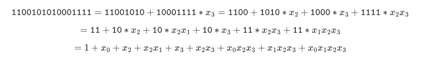
We’re here in $\tau_3$ we can write the full value like this:
$(((x_0 + 1)x_1 + x_0 + 1 )x_2 + (0x_0 + 0)x_1 + 0x_0 + 1 )x_3 + ( (0x_0 + 1)x_1 + 0x_0 + 1 )x_2 + (0x_0 + 0)x_1 + x_0 + 1$

If you look at the coefficient (in reverse), you can see that it corresponds to the coefficients in the example: 1100101010001111
From there you can easily understand how it’s expanded and the bit-string keeps being split in 2.

• First you split the $(...)x_3$ part and the rest:
  $(((x_0 + 1)x_1 + x_0 + 1)x_2 + (0x_0 + 0)x_1 + 0x_0 + 1)x_3$ → 10001111
  $((0x_0 + 1)x_1 + 0x_0 + 1)x_2 + (0x_0 + 0)x_1 + x_0 + 1$ → 11001010
• Then, in both parts, we split again over $(...)x_2$:
  $(((x_0 + 1)x_1 + x_0 + 1)x_2$ → 1111
  $(0x_0 + 0)x_1 + 0x_0 + 1$ → 1000
  $((0x_0 + 1)x_1 + 0x_0 + 1)x_2$ → 1010
  $(0x_0 + 0)x_1 + x_0 + 1$ → 1100
• we we keep going like this until we have just individual parts

Addition

With binary fields, an addition is just a simple XOR.
Let’s give a few examples in $\tau_1$ and $\tau_2$, we can keep going, but then it’s just annoying to do manually
Let’s place ourselves in $\tau_1$:

• $(u)+(u+1)=2u+1=1$
  if we take the bit representation, we have: 01 + 11 = 10
• $(u+1)+(u+1) = 0$ → 11 + 11 = 00

Here’s

+	0	1	u	u + 1
0	0	1	u	u + 1
1	1	0	u + 1	u
u	u	u + 1	0	1
u + 1	u + 1	u	1	0

in bit representation

+	00	10	01	11
00	00	10	01	11
10	10	00	11	01
01	01	11	00	10
11	11	01	10	00

Now let’s try in $\tau_2$:
$((u + 1)v +u) + (uv+1)=uv+v+u+uv+1=v+u+1$
If we take the bit representation, it looks like: 0111 + 1001 = 1110
Again, it checks out with the XOR

Multiplication

x	0	1	u	u + 1
0	0	0	0	0
1	0	1	u	u + 1
u	0	u	u + 1	1
u + 1	0	u + 1	1	u

Table for $\tau_2$

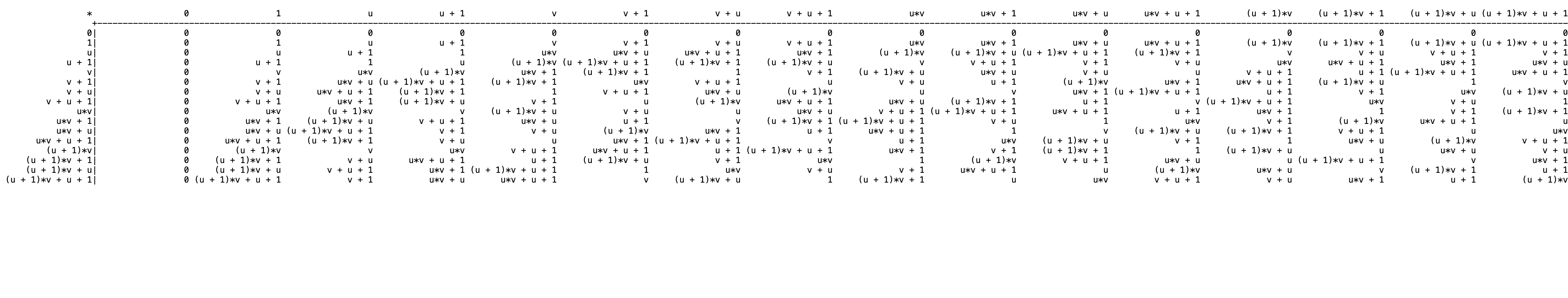
I used Sage to print that table:

print(T_2.multiplication_table("elements"))

Remember how I said at the beginning that we could use “lookup tables”? That’s what I was talking about. But you can also see how fast the lookup table grows. It’s the square of the number of elements in the field. So they should be chosen carefully.
Let’s do one last example manually. I’ll use again u and v because it’s easier to visualize.
We’ll show that $(u*v+1) * ((u+1)v+u) = u*v + u + 1$
$(uv+1) * ((u+1)v+u)$
$= (uv+1) * (uv+v+u)$
$= u^2*v^2 + u*v^2 + u^2*v + u*v + v + u$
$= v^2*(u^2+u) + u^2*v + uv + v + u$

Remember that in $\tau_2$, we have:

• $u^2 = u + 1$
• $v^2 = uv + 1$

$=(uv+1)((u+1)+u) + (u+1)v + uv + v + u$
we can simplify: $u+1+u=2u+1=1$
$=uv + 1 + uv + v + uv + v + u$
$=3uv+2v+u+1$
$=uv+u+1$

Fan-Paar reduction

Throughout the article, I simplified and said that the choice of the irreducible polynomial didn’t matter. I was lying.
Binius uses ${x_k}^2+x_{k-1}x_k+1$ and it’s not random.
This comes from the “Fan-Paar tower” described in the paper “On efficient inversion in tower fields of characteristic two” which allows for much more efficient multiplication and reduction for binary fields.
The key idea is that instead of doing arithmetic in a large extension field $\mathbb{F}_{2^n}$ directly, we recursively break it down into smaller parts until we are left with only operations in the base field. And… we just saw that operations in the base field $\mathbb{F}_2$ are really cheap!
You can find here an example in python of how the algorithm is implemented.

Conclusion

That was a long one! 😰 But I hope you learned a lot!
You’re now a master of binary extension fields $\mathbb{F}_{2^n}$
We now have the knowledge to go on to more advanced topics. In the next article we’ll start looking into Binius and understand how we can create ZK proofs from it.
If something in the article is wrong, or if you have any question, I’ll be happy to answer on Twitter. Don’t hesitate to message me: @0xteddav

Resources

https://vitalik.eth.limo/general/2024/04/29/binius.html
https://blog.lambdaclass.com/climbing-the-tower-field-extensions/
https://hackmd.io/@benjaminion/bls12-381
https://coders-errand.com/zk-snarks-and-their-algebraic-structure-part-4/
https://blog.bitlayer.org/Binius_STARKs_Analysis_and_Its_Optimization/
https://blog.icme.io/small-fields-for-zero-knowledge/
https://eprint.iacr.org/2023/1784.pdf