FRI: A Polynomial Commitment Scheme Explained

Introduction

FRI (Fast Reed-Solomon Interactive Oracle Proof) is a polynomial commitment scheme. Let's break that down:

• Polynomial: If you don't know what this is, this article might not be for you… sorry 😕
• Commitment Scheme: You choose a value and commit to it (e.g., with a hash function). Once committed, you can't change it. Later, you reveal it to prove what you committed to. However, in FRI, you don’t fully reveal it, that’s the magic!
• Polynomial Commitment Scheme: You pick a polynomial and commit to it.

FRI enables a prover to commit to a polynomial and convince a verifier that the polynomial satisfies certain properties, mainly that it has a low degree.

Why Do We Need FRI?

There are several polynomial commitment schemes. What makes FRI special?

• No Trusted Setup ✅ Unlike KZG commitments, which require a structured reference string (SRS), FRI only needs Merkle commitments.
• Post-Quantum Security 🔒 Since it avoids elliptic curve pairings, FRI-based proofs are more resistant to quantum attacks.

Where Is FRI Used?

1. STARKs

FRI is used in STARKs (Scalable Transparent Arguments of Knowledge) to commit to the execution trace of a computation.

2. Data Availability & Danksharding

FRI is also used in data availability sampling. Instead of sending an entire data blob to a client, a validator commits to the data using FRI, and clients can verify data integrity without downloading everything.

Process:

• The original data (e.g., rollup transactions) is structured into a matrix.
• Each row and column undergoes Reed-Solomon encoding, forming a low-degree polynomial for redundancy.
• A commitment is made by evaluating the polynomial on a large domain and constructing a Merkle tree.
• FRI ensures the committed data is close to a low-degree polynomial, confirming correctness.
• Light clients randomly sample portions of the matrix. If these samples match the polynomial, the dataset is likely complete.

Quick description

Before diving into the details, here’s a high-level overview of how FRI works:

1. Start with a polynomial P(x)
2. Choose a domain: for example, values from 1 to 100.
3. Extend the domain using techniques from Reed-Solomon codes.
4. Evaluate P(x) at all points in the extended domain.
5. Build a Merkle tree from these evaluations to commit to them.
6. Perform a verification procedure (involving some "weird computations" 😆) to ensure that P(x) was correctly chosen.

Don’t worry if this seems abstract for now, each step will be explained in detail in the next sections!

What’s this “low degree” thing?

At its core, FRI is all about proving that the initial polynomial has a bounded degree. However, we don’t want to reveal the polynomial itself, so we need a special way to commit to it that convinces the verifier without leaking the entire polynomial and without having to evaluate it entirely.

Step 1: Constructing the Polynomial P(x)

The polynomial P(x) isn’t just any random polynomial, it encodes something specific.

For example, in a STARK proof, P(x) enforces constraints on an execution trace (see the last part of this article: "Bonus: STARK Trace Polynomial"). The entire computation is compiled into this polynomial representation.

To check that P(x) correctly encodes these constraints, we compute its quotient by the zero polynomial. If you’re unfamiliar with this concept, I highly recommend Vitalik’s introduction to SNARKs: Introduction to SNARKs.

Here’s a quick recap:

We want to ensure that P(x) evaluates to 0 over a specific domain, say $x \in [1,9]$

1. Compute the zero polynomial over that domain: $Z(x)=(x-1)(x-2)...(x-9)$
2. If P(x) is correctly enforcing the constraints, then it should be divisible by Z(x) with no remainder. This works because Z(x) is purposefully chosen to be evaluate to zero at those exact points of evaluation
3. This gives us a quotient polynomial

$$Q(x)=\frac{P(x)}{Z(x)}$$

Step 2: Commit and Verify

To commit to P(x), we evaluate P(x), Q(x), and Z(x) over an extended domain.

This is where Reed-Solomon encoding comes in (if you're unfamiliar with it, check out my article: "Reed-Solomon Codes"). It introduces redundancy that prevents cheating, more on that below.

The verifier then picks a random point r from the domain and checks:

$$Q(r)*Z(r)=P(r)$$

Finally, to prevent the prover from tampering with evaluations, we store them in a Merkle tree. If the prover can provide valid Merkle proofs for the values, the verifier is convinced.

Step 3: Why Does Degree Matter?

Since Z(x) is known in advance, we also know that:

$$deg(Q)=deg(P)-deg(Z)$$

And we know in advance the expected degree of P(x).

For example, if the expected degree of P(x) is 100, and we evaluate it over 1000 points: if the prover submits fake polynomials P′ and Q’ of degree ≤ 100, they only have a 10% chance of cheating successfully. Because two polynomials of degree d can match on at most d points.

However, what if they use higher-degree polynomials?

Step 4: How to Cheat With a High-Degree Polynomial

If the prover commits to a polynomial with much higher degree than expected, they can easily bypass the check.

Instead of committing to the correct P(x), they use a fake P’(x). Then, they compute a fake quotient:

$$Q'(i)=\frac{P'(i)}{Z(i)}$$

Since they control P’, they can make sure this condition still holds!

This allows them to pass verification without actually enforcing any constraints, breaking the proof system.

But Q’ will inevitably end up being of degree higher than 100.

Want to see this in action? Check out the script low_degree.sage, where I generate a fake P(x) and trick the verification process. 🚀

Why Must P(x) and Q(x) Be Low-Degree?

The entire security of FRI relies on the fact that P(x) and Q(x) have a bounded degree. If the prover could commit to a high-degree polynomial, they could create a fake quotient Q(x) that satisfies all checks while encoding false or meaningless constraints.

By enforcing a strict degree bound, we ensure that any incorrect polynomial will be detected with high probability, making FRI a sound and reliable way to prove polynomial correctness.

Now, let’s see how it all comes together in practice.

How Does FRI Work?

FRI shifts verification effort from the verifier to the prover. Instead of naively checking all points, the prover commits to polynomials in multiple rounds, and the verifier checks these commitments to detect cheating.

Step 1: Commit (Folding): reducing the polynomial degree

The prover starts with a large polynomial and iteratively reduces its degree in multiple rounds until it reaches a degree that is acceptable for the verifier. This process is a degree reduction step and is a fundamental part of FRI.

At each round, the prover commits to the polynomial by computing a Merkle tree from its evaluations (not coefficients!) at an n-th root of unity.

The Merkle root serves as the commitment, ensuring that the prover cannot change their values later.

Now, let’s see how we transform a polynomial step by step.

Splitting the polynomial into even and odd parts

We start with a polynomial f(x) and split it into its even and odd indexed terms. This allows us to express f(x) in the form:

$$f(x)=f_{even}(x^2)+x*f_{odd}(x^2)$$

Each of these two polynomials has a degree at most half of the original polynomial. This is what allows us to progressively reduce the polynomial's degree.

We’ll use i to indicate the current round, and we’ll call $f_i(x)$ the polynomial at that round.

Example of degree reduction:

$$f_0(x)=7x^4+8x^3+11x^2+5x+2$$

Splitting it into even and odd indexed terms:

$$f_{0/even}(x)=7x^4+11x^2+2 \\ f_{0/odd}(x)=8x^3+5x$$

Rewriting using $x^2$:

$$f_{0/even}(x^2)=7x^2+11x+2 \\ x*f_{0/odd}(x^2)=8x+5$$

Folding with a random scalar alpha

Now, we introduce a random challenge scalar alpha (sent by the verifier) to combine the even and odd parts:

$$f_1(x)=f_{0/even} + \alpha_0 *f_{0/odd}$$

Let’s pick alpha = 5 as an example:

$$f_1(x)=(7x^2+11x+2) + 5*(8x+5)$$

Expanding:

$$f_1(x)=7x^2+51x+27$$

The new polynomial f1(x) has degree reduced by half compared to f0(x).

General formula for each round

At every round i, the prover computes:

$$f_i=f_{i-1/even} + \alpha_{i} *f_{i-1/odd}$$

This process is repeated until the polynomial reaches a sufficiently small degree, making it easy for the verifier to check.

Here’s a simple Sage script to experiment:

def split_polynomial(poly: R) -> tuple[R, R]:
    x = poly.parent().gen()
    coeffs = poly.coefficients(sparse=False)
    deg = poly.degree()
    Pe = R(sum(coeffs[i] * x^(i//2) for i in range(0, deg + 1, 2)))
    Po = R(sum(coeffs[i] * x^((i-1)//2) for i in range(1, deg + 1, 2)))
    return Pe, Po

F = GF(101)
R.<x> = F[]

F0 = 7*x^4 + 8*x^3 + 11*x^2 + 5*x + 2

Fe,Fo=split_polynomial(F0)

alpha = 5
F1 = Fe + alpha*Fo

Pick $\alpha$ from a larger domain

If the base field we’re using is small, challenge $\alpha$ needs to be sampled from a field extension. This prevents the prover from exploiting the small field structure to cheat.

If you need a refresher on field extensions, check out my previous article on extension fields.

We'll first introduce the rest of the FRI process using only the base field. This will help build intuition about how degree reduction and verification work. Later, I'll revisit how the process changes when alpha is sampled from a field extension, and why this is necessary for security when working over small fields.

Step 2: Query

Now that the prover has committed to the polynomial in multiple rounds, the verifier needs to ensure that the prover didn’t cheat. To do this, the verifier picks a random point z and queries $f_i(z)$ and $f_i(-z)$.

If you recall how $f_i(x)$ was computed in the previous step, you’ll notice the following identities hold:

$$f_i(z)=f_{i-1/even}(z^2) + z * f_{i-1/odd}(z^2) \\ f_i(-z)=f_{i-1/even}(z^2) - z * f_{i-1/odd}(z^2)$$

This is easy to verify with code:

z = 17
assert(F0(z) == Fe(z^2) + z*Fo(z^2))
assert(F0(-z) == Fe(z^2) - z*Fo(z^2))

By querying these two values, the verifier ensures that the prover has correctly followed the folding process from $f_{i-1}$ to $f_i$. We’ll see how in the next part, because remember that the verifier doesn’t have access to the even and odd parts.

Finally, the prover also provides a Merkle proof for the queried values at z, allowing the verifier to check their consistency with the original commitment.

This part was easy! Now comes the heavy math for verification. 😱

Step 3: Verification

At each round, the verifier doesn’t have direct access to the even and odd parts of the polynomial. However, using the following key equations, they can verify that the prover's commitments remain consistent from one round to the next:

$$f_{even}(x^2)=\frac{f(x)+f(-x)}{2} \\ f_{odd}(x^2)=\frac{f(x)-f(-x)}{2x}$$

Before diving into why these formulas work, let’s do a quick sanity check in Sage to confirm they hold:

assert(Fe(x^2) == (F0 + F0(-x)) / 2)
assert(Fo(x^2) == (F0 - F0(-x)) / (2 * x))

Why does it work?

The trick lies in how polynomials behave under negation. When evaluating f(-x), the sign flips only for terms with odd-degree exponents, while even-degree terms remain unchanged. This gives us a simple way to separate even and odd components:

• Adding f(x) and f(-x) cancels out all odd terms, leaving only the even-degree terms (multiplied by 2).
• Subtracting f(-x) from f(x) cancels the even terms and isolates the odd terms, but since each odd term originally had an extra x, we divide by 2x to extract them.

Example:

Let’s verify this with an actual polynomial:

$$f(x)=7x^4+8x^3+11x^2+5x+2$$

Evaluating at -x:

$$f(-x) = 7x^4-8x^3+11x^2-5x+2$$

Now applying the formulas:

$$f(x)+f(-x)= 2*(7x^4+11x^2+2) \\ f(x)-f(-x)= 2*(8x^3+5x)=2x*(8x^2+5)$$

Thus, the formulas correctly extract the even and odd parts.

Final verification

Now that we can extract even and odd parts, we can check if the prover has correctly followed the protocol across rounds. The key equation for verification is:

$$f_1(x^2)=\frac{f_0(x)+f_0(-x)}{2}+\alpha_i\frac{f_0(x)-f_0(-x)}{2x}$$

This ensures that the polynomial from the next round ($f_1$) is computed correctly from the previous one ($f_0$). Another quick check in Sage:

assert(F1(x^2) == (F0 + F0(-x))/2 + alpha * ((F0 - F0(-x))/(2*x)))

Naturally, this process generalizes across rounds:

$$f_{i+1}(x^2)=\frac{f_i(x)+f_i(-x)}{2}+\alpha_i\frac{f_i(x)-f_i(-x)}{2x}$$

This equation is often rewritten in an alternative form:

$$f_{i+1}(x^2)=\frac{x+\alpha_i}{2x}f_i(x)+\frac{x-\alpha_i}{2x}f_i(-x)$$

Mathematically, both are equivalent; the second form is just rearranged to highlight the weighting of $f_i(x)$ and $f_i(-x)$.

At this point, we have everything we need to verify that the prover has correctly reduced the polynomial degree across rounds! 🎉

Merkle proof

We just have one extra step: verifying that $f(z)$ and $f(-z)$ were indeed in the Merkle tree.

Since the prover commits to each polynomial at every round using a Merkle tree, the verifier must ensure that the values they received $f(z)$ and $f(-z)$ were not fabricated. This is done by checking the Merkle proof, a sequence of hashes proving that these values are part of the committed polynomial's coefficients.

The prover sends the Merkle proofs for both $f(z)$ and $f(-z)$ , allowing the verifier to recompute the root of the Merkle tree. If the computed root matches the previously committed root, the verifier is assured that these values were indeed derived from the committed polynomial and have not been tampered with.

This step is crucial because without it, a dishonest prover could return fake values that satisfy the verification equations without actually being consistent with the committed polynomial. By enforcing this check, we ensure the integrity of the proof process.

Sage scripts

Of course, you know me, I made a Sage script for the entire process. It should make everything easier to understand: fri.sage

Round-by-round process

To make things even clearer, I created a simplified example where we go through FRI step by step, round by round. This should make it much easier to follow: simple_fri.sage

Let’s go through the code together.

We start with the polynomial we want to commit to:

$$P = 3x^7 + 2x^6 + 10x^5 + 4x^4 + 9x^3 + 13x^2 + 10x + 2$$

We’ll work over $\mathbb{F}_{17}$.

In a real FRI scheme, we evaluate the polynomial over a multiplicative subgroup generated by a root of unity. But to keep things simple, we’ll use the domain D=[0..17].

Each round consists of the following steps:

1. Evaluate the polynomial over the current domain.
2. Pick a random $\alpha$
3. Fold the polynomial to reduce its degree.

We repeat this process until we reach a constant polynomial, which means folding is no longer possible.

To verify that the folding was done correctly:

1. Pick a random index z.
2. Retrieve the evaluations of the polynomial at both z and −z in the corresponding round.
3. Square z and repeat the process for the next round.

Finally, we verify the correctness of the FRI protocol using the equation:

$$f_{i+1}(x^2)=\frac{f_i(x)+f_i(-x)}{2}+\alpha_i\frac{f_i(x)-f_i(-x)}{2x}$$

This ensures that each step in the protocol is consistent with the expected folding process.

That’s all! You should be a FRI expert by now! 🎉🧠

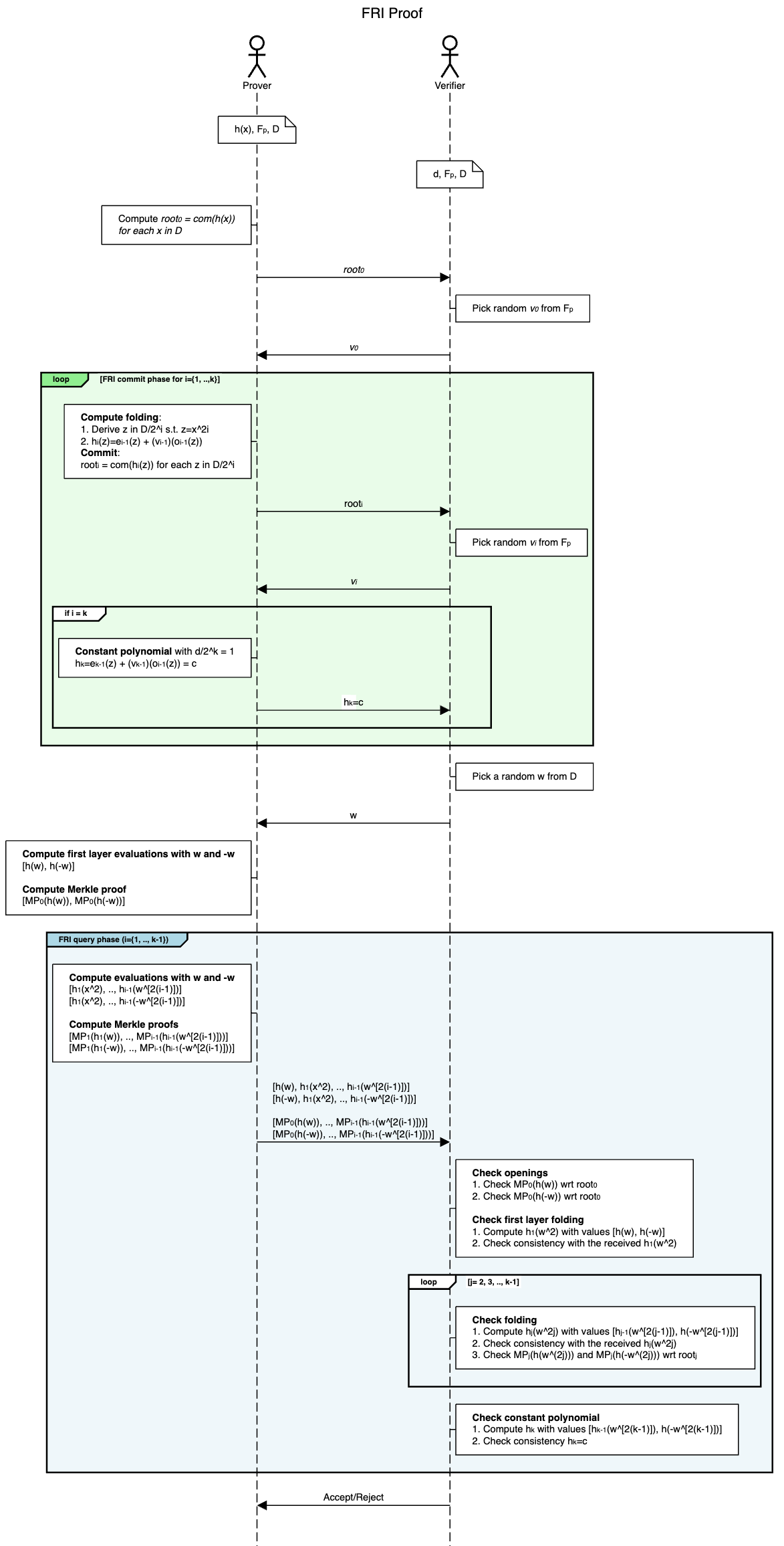
Visual summary

Here’s a great visual summary by Stefano De Angelis from his article Practical notes on the FRI low degree test

Small fields

Earlier, I mentioned that when working over small fields, the challenge $\alpha$ should be sampled from an extension field rather than the base field. This ensures sufficient randomness and prevents certain attacks.

To illustrate this, I wrote another Sage script, which is very similar to the first one, but this time, $\alpha$ is sampled from an extension field: 🔗 fri_ext.sage

In this script, I construct a quadratic extension over $\mathbb{F}_{97}$, defining the field $\mathbb{F}_{{97}^2}$ using the irreducible polynomial

$$x^2 + 96x + 5$$

Since we’re now working with field elements that have two coefficients (like ax + b), we need a way to convert these elements into bytes, for hashing in the Merkle tree.

I added a function ext_to_bytes to handle this conversion. It takes an element v from the extension field and extracts its coefficients, storing them in reverse order (so the constant term b comes first, followed by a): b|a

def ext_to_bytes(v: EXT) -> bytes:
    return "|".join([str(c) for c in v.polynomial().coefficients()]).encode()

This ensures that values from the extension can be consistently hashed and included in the Merkle tree.

Layer 0 openings must be in $\mathbb{F}_{97}$

One important detail: while we sample $\alpha$ from the extension field, the original polynomial f(x) is still defined over the base field $\mathbb{F}$. This means that when the verifier checks the first layer (layer 0) of the Merkle tree, the openings at queried positions must remain in $\mathbb{F}$ and not in the extension field.

Once the FRI folding process begins, we allow intermediate polynomials to have coefficients in the extension field, but we always ensure that the initial values stay in $\mathbb{F}$, keeping the system sound and verifiable.

Bonus: STARK trace polynomial

If we take a step back, where did f(x) come from?

It’s the trace polynomial, which encodes the execution of a computation in STARKs. When a program runs, it produces a sequence of states: this sequence is called the execution trace. Each step of the computation is recorded in a matrix, where each row represents a state of the system and each column represents a specific register or memory value at that step.

To prove that the computation was executed correctly, we encode this trace into polynomials:

1. Execution trace → Polynomials:

The values in each column are interpreted as evaluations of a polynomial over a structured domain

The prover interpolates these values to obtain polynomials that represent the evolution of each register over time.

2. Constraint enforcement:

A set of constraints (e.g., transition rules, boundary conditions) must hold between consecutive rows of the trace.

These constraints are expressed as polynomial equations that must evaluate to zero on the trace polynomials.

3. Commitment & FRI:

The prover commits to these polynomials using Merkle trees, then applies FRI to prove that they are of low degree, ensuring they were generated correctly. The verifier then checks the FRI proof to confirm the integrity of the computation without needing to see the entire execution trace.

STARKs use FRI because it provides a succinct and efficient way to verify that the committed polynomials satisfy the required constraints, without relying on trusted setups or quantum-vulnerable cryptographic assumptions. This makes them ideal for scalable and post-quantum secure proof systems.

Stark by Hand

If you want to dive deeper into STARKs, I highly recommend the STARK by Hand tutorial by Risc0, it’s a fantastic resource! And, of course, to make things even easier to understand and experiment with, I made a Sage script again 😊: https://github.com/teddav/stark_by_hand/blob/main/stark_by_hand.sage

Bonus 2: implementing with Plonky3

To be implemented… 😁

Sorry! I haven’t had time to make this part nicely and well commented yet, so I’ll update it soon.

Resources and Acknowledgements

Thanks @qpzm, @oba and @nico_mnbl for proofreading the article and/or answering my questions about FRI 😊

Great resources:

• ZK Whiteboard Sessions about FRI
  • https://www.youtube.com/watch?v=MBDBrEr2XQg&ab_channel=ZKHack
  • https://www.youtube.com/watch?v=CWbx_rnj7LI&ab_channel=ZKHack
• https://hackmd.io/@deanstef/SJTT3MDhC
• https://medium.com/starkware/low-degree-testing-f7614f5172db
• https://blog.lambdaclass.com/how-to-code-fri-from-scratch/
• https://dev.risczero.com/proof-system/stark-by-hand